My new review in Trends in Ecology and Evolution went live last week. This paper, while not really experimental, took a little bit of a circuitous route and a bit of luck. For all of you out there sitting on ideas for reviews/opinions but not knowing how to get these published, here's how it happened (with a bit of philosophy of how to be a researcher thrown in).
One of the important skills I first learned in grad school was how to delve headfirst into a completely new topic and figure out the salient and relevant points. Sure, you might get sent a paper of interest by a colleague or have one picked for journal club, and these are great for getting a cliff's notes version of an area of research, but to understand a topic you need to know the background. One of the best ways for me to figure out the background (i.e why is the question interesting, what has been done in the past, what are directions for future research) was to find a review article and use that to point towards new references. These references can be found in the articles themselves, but its also quite helpful to search for other articles that cite the review. It doesn't even have to be a new article, because the rabbit hole of references eventually leads to the present day.
Somewhere along the way I developed a soft spot for the Trends family of journals (I know...Elsevier is evil...fully acknowledged, Frontiers is turning into a great place for reviews in the future). Trends articles were clear, concise, opinionated, and a great foothold for jumping into new areas. While there are other equally great resources for reviews like the Annual Reviews family, Bioessays, MMBR, etc...I set it as a goal early on in grad school to publish a first author article in Trends.
There are two different paths to write a Trends article: 1) you can receive an invitation from one of the editors or 2) you can submit a short pre-proposal and see if an Editor likes the idea. I was part of an invited review once, but this new article was the product of submitting and resubmitting pre-proposals.
When I started my lab I wanted to break away from what my postdoctoral advisor (Jeff Dangl) is known for and get back to my roots in microbial evolution. Sure, I still do a lot of phytopathology work in my lab, but I try to do this in the context of understanding how microbial pathogens evolve and adapt to new environments. This strategy has its positives and negatives, but long story short I found myself writing grant applications where the first page was devoted to explaining why the questions I was asking were interesting and important. This was too much space devoted to justifying my questions. Part of this is my lack of grant writing experiences, but part of this was that I felt I had to explain why I was asking the questions I was asking because, while there were many other articles preceding my ideas, there was no article (*as far as I can tell, point me towards these if they exist and I missed them please!) that laid these questions out in the context I was thinking about. I was simply using too many words to say something that could be easier said in a long review article and then cited.
My first stab at getting this review published was a pre-proposal to Trends in Microbiology. Obviously, this didn't work. I took a little bit of time, re-jiggered the ideas and foci, and submitted another pre-proposal to Trends in Ecology and Evolution (TREE). This time a very kind editor thought enough of what I wrote to give me a chance at a full article. I hadn't actually written the article yet, but the ideas were circulating in my head and most of the references I ended up using were gleaned from iterations of grants I was writing. I had about 3 months to write the full article, which is both plenty of time and not close to enough time, but I was able to pull together a draft and circulate it amongst my colleagues before submitting for formal peer review. This piece actually started out as an opinion, simply because I wasn't really sure if people were thinking about things the way I was. There is a feeling in science where you are both terrified and excited in the same moment. Either you are an idiot who is seeing things that other people have seen before and simply don't recognize this, or you are actually seeing things in a new way. The same feeling occurs when dealing with great new experimental results, except there is an extra option...either your experiment is 1) awesome sauce! 2) a trivial result that other people have seen before but which you haven't realized for one reason or another, or 3) a lab mistake.
I got the first reviews back and realized that I was onto something that other people were thinking about already (so...no controversial opinion needed), but that there was definitely a place for what I was writing. It's always difficult to read critique, but the reviewers actually did a great job pointing me towards other papers and helping me discover/emphasize other interesting research findings and directions. Specifically, the first iteration was too heavy on history and specifics and too light on the evolutionary implications of horizontal gene transfer. I made these changes, added a figure (in retrospect, should have changed the font and cut down on whitespace but I'm very happy with the information that it conveys), and sent it back in for a second review. This time it went through without a hitch, and I celebrated accordingly. Side note: I'm a slightly large person and have a tendency to break things in the house and the lab (My wife calls me Shrek). The sequence of the disruptive protein in figure 1 is an homage to my tendencies. A slightly less than subtle Easter egg, but I like trying to put those in my papers (there are plenty more subtle ones in other papers...). I'm also not alone in doing this.
The take home message is not to worry about whether something is good or not, just submit and see what happens. For a long time I was scared/worried about writing pre-proposals to the Trends editors, but it was a fairly seamless process once I went through it. You don't have to wait for the magical email invitation, just take the initiative and see if your idea flies. I'm writing my first grant after the review is out, and it's definitely much easier to write the background now. The last couple of paragraphs of the review also nicely set up some other manuscripts I'll be submitting this summer.
Thursday, May 30, 2013

Tuesday, May 7, 2013
Follow the biology (pt. 5) Season Finale
Yesterday I described assembling a reference genome for Pseudomonas stutzeri strain 28a24, in order to identify causative mutations for a brown colony/culture phenotype which spontaneously popped up while I was playing around with this strain. It's a pretty striking phenotype:

In addition to Illumina data for the reference parent strain, I also received sequencing reads for this brown colony phenotype strain as well as a couple of other independent derivatives of strain 28a24 (which will also be useful in this mutation hunt). There are a variety of programs to align reads to the draft genome assembly, like Bowtie2 and Maq. However, because it's a bit tricky to align reads back to draft genomes and because I'd like to quickly and visually be able to inspect the alignments, I'm going to use a program called Geneious for this post.
The first step is to import the draft assembly into Geneious, and in this case I've collapsed all of the contigs into one fasta read so that they are separated by 100 N's (that way I can tell what contigs I'm artificially collapsing from real scaffolded contigs). Next I import both trimmed Illumina paired read files, and perform a reference assembly vs. the draft genome. In Geneious it's pretty easy to extract the relevant variant information, like places where coverage is 0 (indicating a deletion) or small variants like single nucleotides or insertions/deletions. Here's what the output looks like:
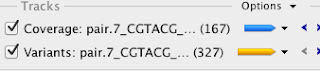
For the reads from the brown phenotype strain there are basically 167 regions where there are no reads mapped back to the draft genome. A quick bit of further inspection shows that these are all just places where I inserted the 100 N's to link together contigs. There are also 327 smaller variants that are backed up with sufficient coverage levels. My arbitrary threshold here was 10 reads per variant, but my coverage levels are way over that across the board (between 70 and 100x).
Here is where those other independent derivatives of the parent strain come into play. There are inevitably going to be assembly errors in the draft genome, and there are going to be places where reads are improperly mapped back to the draft genome. Aligning the independent non-brown isolate reads back against the draft genome and comparing lists of variants allows me to cull the list of variants I need to look more deeply at by disregarding variants shared by both. After this step I'm only left with 3 changes in the brown strain vs. the reference strain.
The first change is at position 2,184,445 in the draft genome, but remember that the number here is arbitrary because I've linked everything together. This variant is a deletion of a G in the brown genome.

Next step is to extract ~1000bp from around the variant and use blastx to give me an idea of what this protein is.
 Basically it's a chemotaxis signaling gene. Not the best candidate for the brown phenotype, but an indication that the brown strain probably isn't as motile as 28a24. Next variant up is at position 3,555,964. It's a G->T transversion potentially involved in choline transport...still not the best candidate for the brown phenotype.

The last variant is the most interesting. It's a T->G transversion in a gene that codes for homogentisate 1,2-dioxygenase (hgmA)


To illustrate the function of this gene, I'm going to pull up the tyrosine metabolism pathway from the KEGG server (hgmA is highlighted in red).

The function of HgmA is to convert homogentisate to 4-Maleyl acetoacetate. Innocuous enough and I'm no biochemist so in pre-Internet world I'd be somewhat lost right now. Luckily I have the power of google and knowledge of the brown phenotype so voila (LMGTFY). Apparently brown pigment accumulation in a wide variety of bacteria is due to a build up of homogentisic acid. There is even this paper in Pseudomonas putida. Oxidation of these compounds leads to quinoid derivatives, which spontaneously polymerize to yield melanin like things. Without doing any more genetics I'm pretty sure this is what I've been looking for. It's a glutamate to an aspartate change at position 338 in the protein sequence, a fairly innocuous change but which is (if this truly is the causal variant) in a very important part of the protein sequence. From here, if I were interested, I would clone the wild type version of hgmA and naturally transform it back into the brown variant of 28a24 to complement the mutation and demonstrate direct causality. I might also try and set up media without tyrosine to see if this strain is auxotrophic, which is a quality of other brown variants (see the P. putida paper above). For now I'll just leave it at that and move on to another interesting project that I can blog about.
In addition to Illumina data for the reference parent strain, I also received sequencing reads for this brown colony phenotype strain as well as a couple of other independent derivatives of strain 28a24 (which will also be useful in this mutation hunt). There are a variety of programs to align reads to the draft genome assembly, like Bowtie2 and Maq. However, because it's a bit tricky to align reads back to draft genomes and because I'd like to quickly and visually be able to inspect the alignments, I'm going to use a program called Geneious for this post.
The first step is to import the draft assembly into Geneious, and in this case I've collapsed all of the contigs into one fasta read so that they are separated by 100 N's (that way I can tell what contigs I'm artificially collapsing from real scaffolded contigs). Next I import both trimmed Illumina paired read files, and perform a reference assembly vs. the draft genome. In Geneious it's pretty easy to extract the relevant variant information, like places where coverage is 0 (indicating a deletion) or small variants like single nucleotides or insertions/deletions. Here's what the output looks like:
For the reads from the brown phenotype strain there are basically 167 regions where there are no reads mapped back to the draft genome. A quick bit of further inspection shows that these are all just places where I inserted the 100 N's to link together contigs. There are also 327 smaller variants that are backed up with sufficient coverage levels. My arbitrary threshold here was 10 reads per variant, but my coverage levels are way over that across the board (between 70 and 100x).
Here is where those other independent derivatives of the parent strain come into play. There are inevitably going to be assembly errors in the draft genome, and there are going to be places where reads are improperly mapped back to the draft genome. Aligning the independent non-brown isolate reads back against the draft genome and comparing lists of variants allows me to cull the list of variants I need to look more deeply at by disregarding variants shared by both. After this step I'm only left with 3 changes in the brown strain vs. the reference strain.
The first change is at position 2,184,445 in the draft genome, but remember that the number here is arbitrary because I've linked everything together. This variant is a deletion of a G in the brown genome.
Next step is to extract ~1000bp from around the variant and use blastx to give me an idea of what this protein is.
The last variant is the most interesting. It's a T->G transversion in a gene that codes for homogentisate 1,2-dioxygenase (hgmA)
To illustrate the function of this gene, I'm going to pull up the tyrosine metabolism pathway from the KEGG server (hgmA is highlighted in red).
The function of HgmA is to convert homogentisate to 4-Maleyl acetoacetate. Innocuous enough and I'm no biochemist so in pre-Internet world I'd be somewhat lost right now. Luckily I have the power of google and knowledge of the brown phenotype so voila (LMGTFY). Apparently brown pigment accumulation in a wide variety of bacteria is due to a build up of homogentisic acid. There is even this paper in Pseudomonas putida. Oxidation of these compounds leads to quinoid derivatives, which spontaneously polymerize to yield melanin like things. Without doing any more genetics I'm pretty sure this is what I've been looking for. It's a glutamate to an aspartate change at position 338 in the protein sequence, a fairly innocuous change but which is (if this truly is the causal variant) in a very important part of the protein sequence. From here, if I were interested, I would clone the wild type version of hgmA and naturally transform it back into the brown variant of 28a24 to complement the mutation and demonstrate direct causality. I might also try and set up media without tyrosine to see if this strain is auxotrophic, which is a quality of other brown variants (see the P. putida paper above). For now I'll just leave it at that and move on to another interesting project that I can blog about.
Monday, May 6, 2013
Follow the biology (pt. 4). Now we are getting somewhere...
First off, apologies on the complete lack of updates. In all honesty, there hasn't been much going on with this project since last summer but now I'm finally at the point of figuring out what kinds of genes are behind this mysterious brown colony phenotype in P. stutzeri.
Picking up where I left off , I've been through many unsuccessful attempts to disrupt the brown phenotype with transposon mutagenesis. The other straightforward option for figuring out the genetic basis for this effect is to sequence the whole genome of the mutant strain and find differences between the mutant and the wild type. Luckily this is 2013 and is easily possible. Confession time, while I know my way around genome scale data and can handle these type of analyses, I am by no means a full fledged bioinformaticist. I'm a microbial geneticist that can run command line unix programs and program a little bit in perl and python, out of necessity. If you have advice or ideas or a better way to carry out the analyses I'm going to describe below, please leave a comment or contact me outside of the blog. I'm always up for learning new and better ways to analyze data!
Long story short, I decided to sequence a variety of genomes using Illumina 100bp PE libraries on a HiSeq. For a single bacterial genome one lane of Illumina HiSeq is complete and utter overkill, when you can multiplex and sequence 24 at a time it's still overkill but less so. In case you are wondering, my upper limit it 24 for this run because of money not because of lack of want. It's a blunt decision, but one of many cost-benefit types of decisions you have to weigh when running a lab on a time dependent budget.
Before I even start to look into the brown mutant genome (next post), the first thing that needs to be done is sequencing and assembly of the reference, "wild type" strain. The bacteria I'm working with here is Pseudomonas stutzeri, specifically strain 28a24 from this paper by Johannes Sikorski. I acquired a murder (not the right collective noun, but any microbiologist can sympathize) of strains from Johannes a few years ago because one of my interests is on the evolutionary effects of natural transformation in natural populations. At the time I had just started a postdoc in Jeff Dangl's lab working with P. syringae, saw the power of Pseudomonads as a system, and wanted to get my hands on naturally transformable strains. Didn't quite know what I was going to do with them at the time, but since I started my lab in Tucson this 28a23 strain has come in very handy as an evolutionary model system.
I received my Illumina read files last week from our sequencing center, and began the slog that can be assembly. While bacterial genome assembly is going to get much easier and exact in the next 5 years (see here) right now working with Illumina reads is kind of like cooking in that you start with a base dish that is seasoned to flavor. My dish of choice for working with Illumina reads is SOAPdenovo. Why you may ask? Frankly, most of the short read assemblers perform equally on bacterial genomes for Illumina PE. Way back when I started using Velvet as an assembler, but over time became frustrated with the implementation. I can't quite recall when it happened, but it might have been when Illumina came out with their GAII platform and the computer cluster I was working with at the time didn't have enough memory to actually assemble genomes with Velvet. Regardless...I mean no slight to Daniel Zerbino and the EMBL team, but at that point I went with SOAPdenovo and have been working with this since due to what I'd like to euphemistically call "research momentum".
Every time I've performed assemblies with 100bp PE reads, the best kmer size for the assemblies always falls around 47 and so I always start around that number and modify as necessary (In case you are curious, helpful tutorials for how De Bruijn graphs work can be found here). One more thing to mention, these reads have already been trimmed for quality. The first thing I noticed with this recent batch of data was that there was A HUGE AMOUNT of it, even when split into 24 different samples. The thing about bacterial genome assemblies is that they start to crap out somewhere above 70 or 80x coverage, basically because depth and random errors confuse the assemblers. If I run the assembler including all of the data, this is the result:
2251 Contigs of 2251 are over bp -> 4674087 total bp
218 Contigs above 5000bp -> 1612110 total bp
30 Contigs above 10000 bp -> 352858 total bp
0 Contigs above 50000 bp -> 0 total bp
0 Contigs above 100,000 bp -> 0 total bp
0 Contigs above 200,000 bp -> 0 total bp
Mean Contig size = 2076.44913371835 bp
Largest Contig = 20517
The output is from a program Josie Reinhardt wrote when she was a grad student in Corbin Jones' lab (used again because of research momentum). The first line gives the total amount of contigs and scaffolds in the assembly, as well as the total assembly size. In this case, including all of the data yields 2251 total contigs, a total genome size of 4.67Mb, and a mean/largest contig of 2076/25,517bp. Not great, but I warned you about including everything.
Next, I'm going to lower the coverage. Judging by this assembly and other P. stutzeri genome sizes, 4.5Mb is right where this genome should be. For 70x or so coverage I am going to only want to include approximately 1.6 million reads from each PE file ( (4,500,000*70) / 200). When I run the assembly this time, the output gets significantly better:
467 Contigs of 467 are over bp -> 4695960 total bp
224 Contigs above 5000bp -> 4375593 total bp
158 Contigs above 10000 bp -> 3890697 total bp
11 Contigs above 50000 bp -> 709014 total bp
0 Contigs above 100,000 bp -> 0 total bp
0 Contigs above 200,000 bp -> 0 total bp
Mean Contig size = 10055.5888650964 bp
Largest Contig = 81785
I can show you more of this type of data with different amounts of coverage, but it's not going to change the outcome. The only other parameter to change a bit is kmer size. The figures above are for 47, but what happens if I use 49 with this reduced coverage?
382 Contigs of 382 are over bp -> 4694856 total bp
178 Contigs above 5000bp -> 4429753 total bp
130 Contigs above 10000 bp -> 4065927 total bp
18 Contigs above 50000 bp -> 1317727 total bp
2 Contigs above 100,000 bp -> 211768 total bp
0 Contigs above 200,000 bp -> 0 total bp
Mean Contig size = 12290.1989528796 bp
Largest Contig = 110167
Even better (and the best assemblies I've gotten so far). Increasing kmer size to 51 makes it incrementally worse:
479 Contigs of 479 are over bp -> 4633694 total bp
164 Contigs above 5000bp -> 4361629 total bp
124 Contigs above 10000 bp -> 4057109 total bp
19 Contigs above 50000 bp -> 1389519 total bp
1 Contigs above 100,000 bp -> 120161 total bp
0 Contigs above 200,000 bp -> 0 total bp
Mean Contig size = 9673.68267223382 bp
Largest Contig = 120161
Picking up where I left off , I've been through many unsuccessful attempts to disrupt the brown phenotype with transposon mutagenesis. The other straightforward option for figuring out the genetic basis for this effect is to sequence the whole genome of the mutant strain and find differences between the mutant and the wild type. Luckily this is 2013 and is easily possible. Confession time, while I know my way around genome scale data and can handle these type of analyses, I am by no means a full fledged bioinformaticist. I'm a microbial geneticist that can run command line unix programs and program a little bit in perl and python, out of necessity. If you have advice or ideas or a better way to carry out the analyses I'm going to describe below, please leave a comment or contact me outside of the blog. I'm always up for learning new and better ways to analyze data!
Long story short, I decided to sequence a variety of genomes using Illumina 100bp PE libraries on a HiSeq. For a single bacterial genome one lane of Illumina HiSeq is complete and utter overkill, when you can multiplex and sequence 24 at a time it's still overkill but less so. In case you are wondering, my upper limit it 24 for this run because of money not because of lack of want. It's a blunt decision, but one of many cost-benefit types of decisions you have to weigh when running a lab on a time dependent budget.
Before I even start to look into the brown mutant genome (next post), the first thing that needs to be done is sequencing and assembly of the reference, "wild type" strain. The bacteria I'm working with here is Pseudomonas stutzeri, specifically strain 28a24 from this paper by Johannes Sikorski. I acquired a murder (not the right collective noun, but any microbiologist can sympathize) of strains from Johannes a few years ago because one of my interests is on the evolutionary effects of natural transformation in natural populations. At the time I had just started a postdoc in Jeff Dangl's lab working with P. syringae, saw the power of Pseudomonads as a system, and wanted to get my hands on naturally transformable strains. Didn't quite know what I was going to do with them at the time, but since I started my lab in Tucson this 28a23 strain has come in very handy as an evolutionary model system.
I received my Illumina read files last week from our sequencing center, and began the slog that can be assembly. While bacterial genome assembly is going to get much easier and exact in the next 5 years (see here) right now working with Illumina reads is kind of like cooking in that you start with a base dish that is seasoned to flavor. My dish of choice for working with Illumina reads is SOAPdenovo. Why you may ask? Frankly, most of the short read assemblers perform equally on bacterial genomes for Illumina PE. Way back when I started using Velvet as an assembler, but over time became frustrated with the implementation. I can't quite recall when it happened, but it might have been when Illumina came out with their GAII platform and the computer cluster I was working with at the time didn't have enough memory to actually assemble genomes with Velvet. Regardless...I mean no slight to Daniel Zerbino and the EMBL team, but at that point I went with SOAPdenovo and have been working with this since due to what I'd like to euphemistically call "research momentum".
Every time I've performed assemblies with 100bp PE reads, the best kmer size for the assemblies always falls around 47 and so I always start around that number and modify as necessary (In case you are curious, helpful tutorials for how De Bruijn graphs work can be found here). One more thing to mention, these reads have already been trimmed for quality. The first thing I noticed with this recent batch of data was that there was A HUGE AMOUNT of it, even when split into 24 different samples. The thing about bacterial genome assemblies is that they start to crap out somewhere above 70 or 80x coverage, basically because depth and random errors confuse the assemblers. If I run the assembler including all of the data, this is the result:
2251 Contigs of 2251 are over bp -> 4674087 total bp
218 Contigs above 5000bp -> 1612110 total bp
30 Contigs above 10000 bp -> 352858 total bp
0 Contigs above 50000 bp -> 0 total bp
0 Contigs above 100,000 bp -> 0 total bp
0 Contigs above 200,000 bp -> 0 total bp
Mean Contig size = 2076.44913371835 bp
Largest Contig = 20517
The output is from a program Josie Reinhardt wrote when she was a grad student in Corbin Jones' lab (used again because of research momentum). The first line gives the total amount of contigs and scaffolds in the assembly, as well as the total assembly size. In this case, including all of the data yields 2251 total contigs, a total genome size of 4.67Mb, and a mean/largest contig of 2076/25,517bp. Not great, but I warned you about including everything.
Next, I'm going to lower the coverage. Judging by this assembly and other P. stutzeri genome sizes, 4.5Mb is right where this genome should be. For 70x or so coverage I am going to only want to include approximately 1.6 million reads from each PE file ( (4,500,000*70) / 200). When I run the assembly this time, the output gets significantly better:
467 Contigs of 467 are over bp -> 4695960 total bp
224 Contigs above 5000bp -> 4375593 total bp
158 Contigs above 10000 bp -> 3890697 total bp
11 Contigs above 50000 bp -> 709014 total bp
0 Contigs above 100,000 bp -> 0 total bp
0 Contigs above 200,000 bp -> 0 total bp
Mean Contig size = 10055.5888650964 bp
Largest Contig = 81785
I can show you more of this type of data with different amounts of coverage, but it's not going to change the outcome. The only other parameter to change a bit is kmer size. The figures above are for 47, but what happens if I use 49 with this reduced coverage?
382 Contigs of 382 are over bp -> 4694856 total bp
178 Contigs above 5000bp -> 4429753 total bp
130 Contigs above 10000 bp -> 4065927 total bp
18 Contigs above 50000 bp -> 1317727 total bp
2 Contigs above 100,000 bp -> 211768 total bp
0 Contigs above 200,000 bp -> 0 total bp
Mean Contig size = 12290.1989528796 bp
Largest Contig = 110167
Even better (and the best assemblies I've gotten so far). Increasing kmer size to 51 makes it incrementally worse:
479 Contigs of 479 are over bp -> 4633694 total bp
164 Contigs above 5000bp -> 4361629 total bp
124 Contigs above 10000 bp -> 4057109 total bp
19 Contigs above 50000 bp -> 1389519 total bp
1 Contigs above 100,000 bp -> 120161 total bp
0 Contigs above 200,000 bp -> 0 total bp
Mean Contig size = 9673.68267223382 bp
Largest Contig = 120161
Last question you might have, since there are other P. stutzeri genomes publicly available, is why not use those and carry out reference guided assembly? I haven't really looked into this much yet, but with some quick analyses it doesn't seem like these genomes are really that similar to one another (~85% nucleotide identity, aside from many presence/absence polymorphisms) so it's not that easy to actually line them up by nucleotide sequence. Maybe better when I've got protein sequences, but that's for another post.
So now I'm ready to compare the brown phenotype genome vs. this assembled draft of 28a24. I know what the answer is, but I'm going to leave that until the next post.
Monday, November 26, 2012
Letters of Recommendation
Ahhh...it's grad/med/dental/etc school application season. For the first time ever I'm sitting down to write multiple letters of recommendation for former students and researchers in my lab. I've now seen the process from all sides: as a prospective undergraduate researcher, as a tenure track PI asked to write letters, and as a grad school admissions committee member. I remember being horribly blindsided by the process as an undergrad (they require 3 letters from DIFFERENT people?) and hope to offer a couple of words of advice for those prospective students.
1. Email me way before the deadline to ask about writing a letter. There is nothing worse than finding out that I have to pop out a letter of recommendation in the next couple of days. My life as a PI is stressful enough that I only survive by making lists of things to get done over the next couple of weeks. If you wait until the last minute, even if I think you have a great future as a post-grad, there is a significant chance I will decline because there aren't enough minutes in the day.
2. If you are a student in my class, don't wait until after the final to introduce yourself. I'm pretty good at remembering names and faces and know who participates in class and who doesn't. If you are ultimately thinking about grad school it's a good idea to participate in discussions in my class and answer questions. Not only does this give me ammo to put in the letter, but it makes a good first impression (which never hurts).
3. Get a good grade in my class. I usually only write letters for students that get A's in my class. I will make exceptions if you are an active participant (see #2) or if you've made a good hearted effort to improve your grade as the semester went on. This doesn't just mean doing better on tests, but it means coming to office hours and showing an interest in the material. I can't say this enough, enthusiasm is one of the greatest assets for prospective students.
4. Help me out. A letter of recommendation is just that...I am writing to back you in your pursuit of higher education. You can help by scheduling meetings to come and talk with me in person, give me a feel for what your interests/goals are. Let me know why you want to go to grad school. Tell me stories that illustrate why I should give you my seal of approval. A letter can be pretty dry if all I can write is that you got an A in my class. Seriously, help a brother out here, it will go a long way towards making your letter the best it can be.
5. Don't make me search for addresses to email the letter to or websites to log in to. Please, give me the links and I promise you that it will get done much faster and more smoothly.
6. Ask if there are spots for undergraduate researchers in my lab. There is nothing better in a letter of recommendation for grad school than positive comments about a student's laboratory skills and dedication. All grad school is is trying to figure out how to make experiments work, and you've got a good head start if you've already had this experience. Obviously, the earlier you do this the better.
7. Remember, I'm doing this to help you. There is nothing in my contract that requires me to write letters of recommendation. Seriously, this is a favor I'm doing for you.
Have to write letters? Check this out.
Any other thoughts? Feel free to contribute in the comments.
1. Email me way before the deadline to ask about writing a letter. There is nothing worse than finding out that I have to pop out a letter of recommendation in the next couple of days. My life as a PI is stressful enough that I only survive by making lists of things to get done over the next couple of weeks. If you wait until the last minute, even if I think you have a great future as a post-grad, there is a significant chance I will decline because there aren't enough minutes in the day.
2. If you are a student in my class, don't wait until after the final to introduce yourself. I'm pretty good at remembering names and faces and know who participates in class and who doesn't. If you are ultimately thinking about grad school it's a good idea to participate in discussions in my class and answer questions. Not only does this give me ammo to put in the letter, but it makes a good first impression (which never hurts).
3. Get a good grade in my class. I usually only write letters for students that get A's in my class. I will make exceptions if you are an active participant (see #2) or if you've made a good hearted effort to improve your grade as the semester went on. This doesn't just mean doing better on tests, but it means coming to office hours and showing an interest in the material. I can't say this enough, enthusiasm is one of the greatest assets for prospective students.
4. Help me out. A letter of recommendation is just that...I am writing to back you in your pursuit of higher education. You can help by scheduling meetings to come and talk with me in person, give me a feel for what your interests/goals are. Let me know why you want to go to grad school. Tell me stories that illustrate why I should give you my seal of approval. A letter can be pretty dry if all I can write is that you got an A in my class. Seriously, help a brother out here, it will go a long way towards making your letter the best it can be.
5. Don't make me search for addresses to email the letter to or websites to log in to. Please, give me the links and I promise you that it will get done much faster and more smoothly.
6. Ask if there are spots for undergraduate researchers in my lab. There is nothing better in a letter of recommendation for grad school than positive comments about a student's laboratory skills and dedication. All grad school is is trying to figure out how to make experiments work, and you've got a good head start if you've already had this experience. Obviously, the earlier you do this the better.
7. Remember, I'm doing this to help you. There is nothing in my contract that requires me to write letters of recommendation. Seriously, this is a favor I'm doing for you.
Have to write letters? Check this out.
Any other thoughts? Feel free to contribute in the comments.
Thursday, November 15, 2012
Co-corresponding authors
I was involved in a bit of a discussion over twitter this morning over the value of co-corresponding authors on manuscripts. This has inspired a Drugmonkey blog post with some good comments. Because I've actually published a paper with co-corresponding authors (here), I thought that I could provide a slightly different insight into the process.
First off, what does it mean to be a corresponding author? Traditionally, the corresponding author spot on a paper is there in case researchers stumble across your manuscript and have questions or requests for reagents. This has morphed into somewhat of a status symbol with the increase in number of authors on papers because corresponding authors are seen as having "ownership" (for lack of a better word) over the published project. For instance, in the CV for my tenure packet I list where I am the corresponding author on manuscripts from my own lab that my postdoctoral advisor is also an author on. Maybe this matters, maybe it doesn't, but I see it as a way to point out projects that I have taken more of a lead role on.
So after that brief intro, here's my experience with co-corresponding authorship. Back in 2009 we published a paper on sequencing and assembly of a Pseudomonas syringae strain (here). This paper included biological data as well as a computational pipeline to that we used to assemble the genome. My postdoctoral advisor, Jeff Dangl, was the sole corresponding author on this paper. Jeff is an incredible biologist, but is not the best programmer in the world. Dangl was the perfect corresponding author for any biological question (strain/construct requests, etc...) from that paper. However, Jeff would get emailed questions concerning the computational pipeline and inevitably would forward the emails to the people (Corbin Jones and me) that could actually answer them. This was a bit frustrating.
To prevent this situation in our next paper in this series, which expanded this pipeline and analyses across 19 strains, both Corbin and Dangl were corresponding authors with a note that Jeff would handle the biology and Corbin would handle the computational questions.
One important thing to note...in each case the lead author has been the one actually formatting and uploading the paper to the journal, and also dealt with actual correspondance to the editor of the journal after submission without being listed as corresponding author. As many know, those are the most fun and fulfilling parts of manuscript submission...
First off, what does it mean to be a corresponding author? Traditionally, the corresponding author spot on a paper is there in case researchers stumble across your manuscript and have questions or requests for reagents. This has morphed into somewhat of a status symbol with the increase in number of authors on papers because corresponding authors are seen as having "ownership" (for lack of a better word) over the published project. For instance, in the CV for my tenure packet I list where I am the corresponding author on manuscripts from my own lab that my postdoctoral advisor is also an author on. Maybe this matters, maybe it doesn't, but I see it as a way to point out projects that I have taken more of a lead role on.
So after that brief intro, here's my experience with co-corresponding authorship. Back in 2009 we published a paper on sequencing and assembly of a Pseudomonas syringae strain (here). This paper included biological data as well as a computational pipeline to that we used to assemble the genome. My postdoctoral advisor, Jeff Dangl, was the sole corresponding author on this paper. Jeff is an incredible biologist, but is not the best programmer in the world. Dangl was the perfect corresponding author for any biological question (strain/construct requests, etc...) from that paper. However, Jeff would get emailed questions concerning the computational pipeline and inevitably would forward the emails to the people (Corbin Jones and me) that could actually answer them. This was a bit frustrating.
To prevent this situation in our next paper in this series, which expanded this pipeline and analyses across 19 strains, both Corbin and Dangl were corresponding authors with a note that Jeff would handle the biology and Corbin would handle the computational questions.
One important thing to note...in each case the lead author has been the one actually formatting and uploading the paper to the journal, and also dealt with actual correspondance to the editor of the journal after submission without being listed as corresponding author. As many know, those are the most fun and fulfilling parts of manuscript submission...
Monday, September 24, 2012
Chasing Down the Cause of Random Experimental Results
I'm pretty sure that every wet lab biologist has a story or two or many about experimental controls behaving weirdly or in seemingly unexplainable ways. A very small percentage of the time, chasing down the underlying cause can actually lead to a Nobel prize. Much more often the underlying cause is unremarkable ("Oh, that was a ug instead of mg?"). We had one of these results in the lab last week and, while interesting and actually a real phenomenon rather than facepalmish error, it's still fairly unremarkable so I figure I'd share it here.
We are currently trying to measure mutation rates to rifampicin resistance in Pseudomonas stutzeri. We already have encouraging results showing how a particular genotypic change increases mutation rates to streptomycin resistance and to goal is to calculate mutation rates an additional phenotype so we could begin to think that the genotypic change generally increases mutation rates. For other reasons, we wanted to measure the mutation rates to rifampicin resistance in a streptomycin resistant background strain.
Since P. stutzeri is competent for natural transformation, we transformed a rif and strep sensitive strain (rifS and strepS hereafter) using genomic DNA from a rif and strep resistant strain (rifR and strepR). No problem yet as we got plenty of strepR colonies back.
The next step is to use a fluctuation test to calculate mutation rates to rifR using cultures started from a single strepR colony. The basic idea of a fluctuation test is to grow many independent cultures starting from very low cell densities (typically ~1000 cells, in order to insure that there are no rifR colonies at the start), and then plate the entirety of these cultures under selective conditions once the cultures have grown to appreciable densities. If there are no rifR cells at the beginning of growth , you can use the distribution of rifR colonies that appear across the independent cultures in order to calculate mutation rates.
The picture below describes what you might expect from a typical fluctuation test.

When you plate out samples at time 0, there should be no rifR colonies (which I'm showing as blue circles if present). After growth, in this case 24 hours, rifR cells will have arisen by spontaneous mutation INDEPENDENTLY in each culture. As you can see from the picture, the expectation is that some cultures will not contain any rifR cells, some will have a few, and some will contain many rifR colonies. Those with many colonies are called "jackpots"and may appear as confluent lawns, hence the totality of blue in the picture. There is a distribution of rifR cells across independent cultures because mutations that lead to rifampicin resistance will occur at different points of the growth curve in each culture. A single mutation that arises during the first cell division after starting the experiment will lead to jackpots because these rifR cells have the chance to divide many times before plating. A rifR cell that arises during the last division before plating will only be represented by one colony because it hasn't had the time or resources to divide and proliferate. You can use this distribution to actually figure out mutation rates. Here is Stan Maloy's explanation of the fluctuation test.
Back to our P. stutzeri experiments...when we plated out the fluctuation test for our (what we thought) strepR rifS isolate, we got this result back from the time zero plate.

There was a lawn of rifR bacteria, which is statistically higher than zero (not really, but go with me on this). Even though the mutation rate to rifR is relatively high, something was fishy here because there should have been no colonies. We went back to the original plate of strepR transformants, and streaked additional isolates to both strep and rif plates. Even though the strain which we had originally transformed was rifS, I was surprised when roughly half of the strepR transformants were also rifR.
What could explain this result? The mutations that give rise to the strepR phenotype usually occur within a gene called rpsL. This gene codes for one of the many proteins that make up bacterial ribosomes, and indeed, the mechanism of action for streptomycin is inhibition of translation. The first thing I did was investigate the genomic context, what genes surround rpsL, within the one previously sequenced P. stutzeri genome. Here's what I found at the Pseudomonas genome database (which is extremely handy BTW).

All annotated genes in this section of the P. stutzeri genome are represented as red boxes. rpsL is the red box surrounded by a very dark line. The numbers on the bottom of the picture display the position of each gene in the P. stutzeri genome (rpsL is roughly at position 888,000 out of ~4,000,000). Here's where it gets interesting. Mutations that lead to rifampicin resistance typically occur in a gene called rpoB. This codes for a subunit of RNA polymerase, which makes sense (again) because the mechanism of action for rifampicin is to inhibit transcription. As I described above, we originally made the strepR strain by transforming a rifS strepS strain with genomic DNA from a rifR strepR strain. rpoB and rpsL are only about 5000 bp apart and I originally had no clue that rpoB and rpsL were genomic neighbors. Since, during natural transformation, genomic fragments sized 5Kb and above can be recombined into the recipient genome I'm guessing that a substantial fraction of the cells recombined both strepR and rifR mutations during this step from the donor genomic DNA. Since the exact positions of recombination are essentially random, cells that remained rifS after transformation must have recombined smaller fragments that only contained the strepR mutation. Here's a quick picture of what I think happened.

Rifampicin resistance is colored red, streptomycin resistance is colored blue. Cells that are rifR strepR are colored purple. While there were likely rifR strepS cells generated after transformation, these won't grow on the strepR plate so that's why there aren't red colonies. Mystery solved...and this maybe something I can utilize in future experiments although as of right now I have no idea how. If we would have originally picked a rifS strepR colony for the fluctuation test, I wouldn't have realized any of this. Sometimes science is random.
We are currently trying to measure mutation rates to rifampicin resistance in Pseudomonas stutzeri. We already have encouraging results showing how a particular genotypic change increases mutation rates to streptomycin resistance and to goal is to calculate mutation rates an additional phenotype so we could begin to think that the genotypic change generally increases mutation rates. For other reasons, we wanted to measure the mutation rates to rifampicin resistance in a streptomycin resistant background strain.
Since P. stutzeri is competent for natural transformation, we transformed a rif and strep sensitive strain (rifS and strepS hereafter) using genomic DNA from a rif and strep resistant strain (rifR and strepR). No problem yet as we got plenty of strepR colonies back.
The next step is to use a fluctuation test to calculate mutation rates to rifR using cultures started from a single strepR colony. The basic idea of a fluctuation test is to grow many independent cultures starting from very low cell densities (typically ~1000 cells, in order to insure that there are no rifR colonies at the start), and then plate the entirety of these cultures under selective conditions once the cultures have grown to appreciable densities. If there are no rifR cells at the beginning of growth , you can use the distribution of rifR colonies that appear across the independent cultures in order to calculate mutation rates.
The picture below describes what you might expect from a typical fluctuation test.

When you plate out samples at time 0, there should be no rifR colonies (which I'm showing as blue circles if present). After growth, in this case 24 hours, rifR cells will have arisen by spontaneous mutation INDEPENDENTLY in each culture. As you can see from the picture, the expectation is that some cultures will not contain any rifR cells, some will have a few, and some will contain many rifR colonies. Those with many colonies are called "jackpots"and may appear as confluent lawns, hence the totality of blue in the picture. There is a distribution of rifR cells across independent cultures because mutations that lead to rifampicin resistance will occur at different points of the growth curve in each culture. A single mutation that arises during the first cell division after starting the experiment will lead to jackpots because these rifR cells have the chance to divide many times before plating. A rifR cell that arises during the last division before plating will only be represented by one colony because it hasn't had the time or resources to divide and proliferate. You can use this distribution to actually figure out mutation rates. Here is Stan Maloy's explanation of the fluctuation test.
Back to our P. stutzeri experiments...when we plated out the fluctuation test for our (what we thought) strepR rifS isolate, we got this result back from the time zero plate.

There was a lawn of rifR bacteria, which is statistically higher than zero (not really, but go with me on this). Even though the mutation rate to rifR is relatively high, something was fishy here because there should have been no colonies. We went back to the original plate of strepR transformants, and streaked additional isolates to both strep and rif plates. Even though the strain which we had originally transformed was rifS, I was surprised when roughly half of the strepR transformants were also rifR.
What could explain this result? The mutations that give rise to the strepR phenotype usually occur within a gene called rpsL. This gene codes for one of the many proteins that make up bacterial ribosomes, and indeed, the mechanism of action for streptomycin is inhibition of translation. The first thing I did was investigate the genomic context, what genes surround rpsL, within the one previously sequenced P. stutzeri genome. Here's what I found at the Pseudomonas genome database (which is extremely handy BTW).

All annotated genes in this section of the P. stutzeri genome are represented as red boxes. rpsL is the red box surrounded by a very dark line. The numbers on the bottom of the picture display the position of each gene in the P. stutzeri genome (rpsL is roughly at position 888,000 out of ~4,000,000). Here's where it gets interesting. Mutations that lead to rifampicin resistance typically occur in a gene called rpoB. This codes for a subunit of RNA polymerase, which makes sense (again) because the mechanism of action for rifampicin is to inhibit transcription. As I described above, we originally made the strepR strain by transforming a rifS strepS strain with genomic DNA from a rifR strepR strain. rpoB and rpsL are only about 5000 bp apart and I originally had no clue that rpoB and rpsL were genomic neighbors. Since, during natural transformation, genomic fragments sized 5Kb and above can be recombined into the recipient genome I'm guessing that a substantial fraction of the cells recombined both strepR and rifR mutations during this step from the donor genomic DNA. Since the exact positions of recombination are essentially random, cells that remained rifS after transformation must have recombined smaller fragments that only contained the strepR mutation. Here's a quick picture of what I think happened.

Rifampicin resistance is colored red, streptomycin resistance is colored blue. Cells that are rifR strepR are colored purple. While there were likely rifR strepS cells generated after transformation, these won't grow on the strepR plate so that's why there aren't red colonies. Mystery solved...and this maybe something I can utilize in future experiments although as of right now I have no idea how. If we would have originally picked a rifS strepR colony for the fluctuation test, I wouldn't have realized any of this. Sometimes science is random.
Friday, September 7, 2012
How I came to work with plant pathogens
It's getting to be grant season for me again, and one of the most important parts about writing grants is learning how to sell and justify your research story to a larger (somewhat less specialized) audience. I've also seen some stirrings on blogs and twitter about how to choose postdoc labs and research programs in order to set up an academic career. Although I think that the best answers to the postdoc question are much more dependent on both the individual and the lab, both of these topics inspired me to jot down some ramblings about how my own research program developed.
I've always been interested in understanding how microbial populations adapt to new environments and my graduate school career was spent studying evolutionary dynamics of the human pathogen Helicobacter pylori. Dr. Karen Guillemin had just started her lab at the University of Oregon and I'm most thankful that she was willing to take a chance on having an evolutionary biologist play around in her lab, which at the time was much more focused on understanding the molecular biology of bacterial pathogenesis. I was lucky to be co-advised by Dr. Patrick Phillips (a nematode guy), to fill in the blanks when it came to evolutionary biology, population genetics, and random Star Wars references. My grad school experiments centered around setting up a laboratory evolution system, modeled around the wonderful work of Rich Lenski, where I could test for the effects of genetic exchange on rates of adaptation. I'll talk about the ins and outs of those experiments in a future post, but at the end of graduate school I was left with a huge choice as to where to do my postdoc.At this time experimental evolution was exploding as a research field, and I wanted to continue studying bacterial adaptation using experimental evolution, but I also wanted to begin to study populations within hosts. I actually had a great interview with Rich Lenski in February 2006 in East Lansing where we talked about teaming up with Jeff Gordon at WashU to look at the effects of Rich's E. coli laboratory mutations during mouse infections (among other things including college basketball). After that interview, I was almost convinced that I was going to become a Michigan state Spartan.
There was a counter-voice in the back of my head, however, that maybe I should jump a little bit more out of my experimental comfort zone. I was feeling leery of working with mammalian pathogens for a variety of reasons: 1) I'm a fan of cute fuzzy animals like ferrets, and it would be very difficult for me to actually do research within hosts 2) Coming out of the Phillips lab I was well schooled in the importance of sample size for statistics. It's very expensive to perform large numbers of infections in anything with 4 legs and hair, and I was worried about getting high enough numbers of replicates to actually make sense of evolutionary trends. I knew I wanted to continue on in academia, and I had a serious internal discussion about how easy it would be to fund a lab that performed the experiments with mice that I was imagining. 3) I had a sneaky suspicion that genomics was about to explode (indeed, it already was in 2006), and I wanted to jump on the train. I certainly could have done this in Rich's lab but even at that point the field of the genomics of mammalian pathogens was getting crowded.
So what was my other option? I miraculously came across a random paper out of Jeff Dangl's lab, and had never heard of Dangl before this point (looking back...the only name I recognized on the paper was Dave Guttman from his work on recombination). I shot a quick email off to JD laying out my interests and and was pleasantly surprised that he was willing to fly me out for an interview in Chapel Hill. This interview was scheduled to be a couple of weeks after my interview in Michigan (in February). While can't say that the contrast in weather consciously affected my decision, it was 20 degrees and snowy in Michigan and 70 degrees and sunny in North Carolina during my visits. Dangl was well known in plant biology circles at that time for helping to work out the genetics of plant immune responses to pathogens, indeed, he was elected to the National Academy a couple of years later. Jeff was embarking on a pretty ambitious (as with seemingly all Dangl lab research) project to use "next-generation" sequencing technologies to illuminate genomic diversity in phylogenetically divergent strains of the plant pathogen Pseudomonas syringae. I knew that P. syringae was related to Pseudomonas fluorescens, which is a popular system for experimental evolution studies thanks to Paul Rainey and colleagues, and I figured that I might be able to piggy-back off of that system to set up my own P. syringae evolution experiments one day. This has actually proven to be spot on:) A postdoc at UNC would also throw me into the fire of bacterial genomics and force me to learn how to sequence and assemble strains, perform genomic level experiments, and PROGRAM! Perhaps most importantly, plants grow in dirt (which is dirt cheap) and no one really cares how or how many plants you euthanize during experiments so long as any transgenes stay contained. Working with plant pathogens would enable me to carry out an appropriate number of replicates to try and silence the subtle voice of Patrick Phillips that remains in my head today when I think about statistics and experimental design.
One other helpful piece of evidence that sealed the deal for me to join the Dangl lab was learning that mammalian and plant pathogens pretty much deploy the same sets of tools during pathogenesis. Evolutionary patterns from one system are very similar to the other and research findings are relevant across both, I wasn't really going to miss much studying plant pathogens instead of Shigella. For instance, the importance of type III secretion systems during infection was actually recognized at about the same time for both Yersinia pestis and P. syringae! The similarities have been laid out clearly in paper form a couple of times (here, here, here, here, here, among others) but the main differences between systems arise when immune responses in the hosts are compared. Even then, innate immunity is still a major shared component that contributes significantly to defense responses. As such I'm able to apply for grants across the main funding agencies (NSF, USDA, NIH), which theoretically makes make my life as a PI a little bit easier, although it hasn't yet:)
To be completely honest with you, I was torn after visiting both labs and took a couple of weeks to make my decision. What finally did it for me was flipping a coin, not once or twice, but until there was a run of the same side. UNC came up as the answer about 5 times in a row, and I found myself completely OK with that decision. Sometimes you just have to jump in and not look back.
I've always been interested in understanding how microbial populations adapt to new environments and my graduate school career was spent studying evolutionary dynamics of the human pathogen Helicobacter pylori. Dr. Karen Guillemin had just started her lab at the University of Oregon and I'm most thankful that she was willing to take a chance on having an evolutionary biologist play around in her lab, which at the time was much more focused on understanding the molecular biology of bacterial pathogenesis. I was lucky to be co-advised by Dr. Patrick Phillips (a nematode guy), to fill in the blanks when it came to evolutionary biology, population genetics, and random Star Wars references. My grad school experiments centered around setting up a laboratory evolution system, modeled around the wonderful work of Rich Lenski, where I could test for the effects of genetic exchange on rates of adaptation. I'll talk about the ins and outs of those experiments in a future post, but at the end of graduate school I was left with a huge choice as to where to do my postdoc.At this time experimental evolution was exploding as a research field, and I wanted to continue studying bacterial adaptation using experimental evolution, but I also wanted to begin to study populations within hosts. I actually had a great interview with Rich Lenski in February 2006 in East Lansing where we talked about teaming up with Jeff Gordon at WashU to look at the effects of Rich's E. coli laboratory mutations during mouse infections (among other things including college basketball). After that interview, I was almost convinced that I was going to become a Michigan state Spartan.
There was a counter-voice in the back of my head, however, that maybe I should jump a little bit more out of my experimental comfort zone. I was feeling leery of working with mammalian pathogens for a variety of reasons: 1) I'm a fan of cute fuzzy animals like ferrets, and it would be very difficult for me to actually do research within hosts 2) Coming out of the Phillips lab I was well schooled in the importance of sample size for statistics. It's very expensive to perform large numbers of infections in anything with 4 legs and hair, and I was worried about getting high enough numbers of replicates to actually make sense of evolutionary trends. I knew I wanted to continue on in academia, and I had a serious internal discussion about how easy it would be to fund a lab that performed the experiments with mice that I was imagining. 3) I had a sneaky suspicion that genomics was about to explode (indeed, it already was in 2006), and I wanted to jump on the train. I certainly could have done this in Rich's lab but even at that point the field of the genomics of mammalian pathogens was getting crowded.
So what was my other option? I miraculously came across a random paper out of Jeff Dangl's lab, and had never heard of Dangl before this point (looking back...the only name I recognized on the paper was Dave Guttman from his work on recombination). I shot a quick email off to JD laying out my interests and and was pleasantly surprised that he was willing to fly me out for an interview in Chapel Hill. This interview was scheduled to be a couple of weeks after my interview in Michigan (in February). While can't say that the contrast in weather consciously affected my decision, it was 20 degrees and snowy in Michigan and 70 degrees and sunny in North Carolina during my visits. Dangl was well known in plant biology circles at that time for helping to work out the genetics of plant immune responses to pathogens, indeed, he was elected to the National Academy a couple of years later. Jeff was embarking on a pretty ambitious (as with seemingly all Dangl lab research) project to use "next-generation" sequencing technologies to illuminate genomic diversity in phylogenetically divergent strains of the plant pathogen Pseudomonas syringae. I knew that P. syringae was related to Pseudomonas fluorescens, which is a popular system for experimental evolution studies thanks to Paul Rainey and colleagues, and I figured that I might be able to piggy-back off of that system to set up my own P. syringae evolution experiments one day. This has actually proven to be spot on:) A postdoc at UNC would also throw me into the fire of bacterial genomics and force me to learn how to sequence and assemble strains, perform genomic level experiments, and PROGRAM! Perhaps most importantly, plants grow in dirt (which is dirt cheap) and no one really cares how or how many plants you euthanize during experiments so long as any transgenes stay contained. Working with plant pathogens would enable me to carry out an appropriate number of replicates to try and silence the subtle voice of Patrick Phillips that remains in my head today when I think about statistics and experimental design.
One other helpful piece of evidence that sealed the deal for me to join the Dangl lab was learning that mammalian and plant pathogens pretty much deploy the same sets of tools during pathogenesis. Evolutionary patterns from one system are very similar to the other and research findings are relevant across both, I wasn't really going to miss much studying plant pathogens instead of Shigella. For instance, the importance of type III secretion systems during infection was actually recognized at about the same time for both Yersinia pestis and P. syringae! The similarities have been laid out clearly in paper form a couple of times (here, here, here, here, here, among others) but the main differences between systems arise when immune responses in the hosts are compared. Even then, innate immunity is still a major shared component that contributes significantly to defense responses. As such I'm able to apply for grants across the main funding agencies (NSF, USDA, NIH), which theoretically makes make my life as a PI a little bit easier, although it hasn't yet:)
To be completely honest with you, I was torn after visiting both labs and took a couple of weeks to make my decision. What finally did it for me was flipping a coin, not once or twice, but until there was a run of the same side. UNC came up as the answer about 5 times in a row, and I found myself completely OK with that decision. Sometimes you just have to jump in and not look back.
Subscribe to:
Posts (Atom)